Metamimetism in Spatial Games

Annexe 2

A Detailed Study of a meta-mimetic game

The aim of Annexe 1 is to give more details for the game presented as an example in Metamimetic Games. Altough this king of metamimetic games are very simple, it gives a good insight of the topic. We are here in the following settings :

Matrix Game	C	D		Population size : 10 000	Self-Interaction	initial distribution of imitation rules: uniform		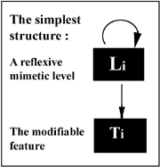	Article on these simulations
C	1	0
D	b	0

with b=1.9 and an initial rate of cooperation among population of Ci=0.5.

We have here parameters of a chaotic regime in the original model (cf annexe 1). Contrary to what happen in the case of a society with only Maxi-agents, there is no chaotic regime but rather an organisation of the network with specific structuresfor each rule for imitation.

The following graphs show the evolution of a particular simulation. Most simulation results are shown until time step 300 since dynamics don't change any more after this time. The most interesting phenomena take place at the beginning. The first striking thing is that the system reaches very quickly its unique attractor (20 periods), which is mostly static (for a 10000 agent population, about a hundred oscillators at the level of imitation rules, less than a dozen at the behavioral level (see fig 1). In the following, we will first adopt a local point of view, looking at a particular agent oscillating between several rules for imitation. We will then have a global approach with statistics on the whole population.

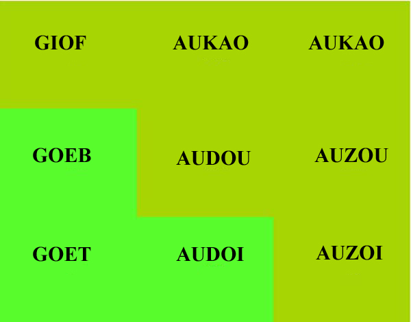
The particular case of AUDOU

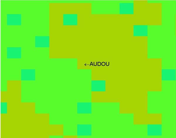
As is was mentionned above, there is still few agents which keep changing their rules for imitation or their actions even after the system has reached its attractor. To understand this phenomenon, we will take the particular case of agent AUDOU. AUDOU is a D-agent which always hesitate between adopting the conformist rule or the Maxi rule. As it can be seen on figure 2, AUDOU is at the border between an conformist area and a Maxi area.

Figure 2-a : AUDOU neighbors.	Figure 2-b : AUDOU, a Maxi-agent is at the border between an conformist area and a Maxi area. Blue squares are minority-agents.

During the time AUDOU keep changing her mind about how she should choose her action, passing from a Maxi rule to an conformist rule an so on (fig 2). It is easy from fig2-a to guess why AUDOU can't keep the conformist rule : in her neighborhood, conformist-agents are always in minority so that if she adopt the conformist rule, she will change her rule for the majoritarian rule in the next update. This is confirmed by study of the evolution of proportions of the different rules in the neighborhood of AUDOU with time (fig3).
To understand why AUDOU cannot keep the Maxi choice, we need to look at AUDOU's neighbors payoffs (fig 4 ). What can be seen, is that there are two agents in AUDOU's neighborhood which are always more successful than AUDOU : AUDOI and AUZOI. Thus, when AUDOU applies the Maxi rule, she imitates randomly one of these two agents (since they both have the same payoffs 2). This explains how AUDOU can choose anconformist rule while beeing adopting the Maxi rule. We can see here that the topology of the social network is crucial for this kind of phenomena. It is precisely because AUDOU wants to imitate some neighbors without having the same neighborhood and thus, the same information, that she always hesitate between two rules. The fact that this kind of configurations can only happen at the border between two areas (of homogenous behaviors or metarules) with the fact that the whole population is strongly structured explains why there are so few oscillators.

 

A Statistical Study of the Dynamics.

The first interesting thing to look at is the frequencies of the different types of rules for imitation (fig 5 ):

1. The majority rule conformist is actually the most common in the population at the attractor. This can be understood by the fact that the higher is the proportion of conformist, the higher is the probability that an conformist agent will be surrounded by a majority of conformist agents, which will make her keep the conformist choice. conformist is self-reinforcing at the population level.
2. Maxi agents form clusters in the conformist Sea. Since locally they are actually the ones winning the more, they don’t change their type.
3. Non Conf. agents are scattered on all the territory (small dots). Their proportion starting from 25% has decreased until each Non Conf. agent is actually in minority in her neighborhood. Non Conf. don’t change their type at the attractor.
4. PDR agents have completely disappeared. Since for a stochastic rule there are always agents changing their type for the type of some neighbor, when the other three types have found stable configurations, the proportion of PDR keep decreasing until it reaches 0.

Even if this model is a very simple application of our formalism, it is good news that conformist is actually a very common rule at the attractorj, since conformism seems to be one of the most common rule in human behaviours.

If we now look at the spatial distribution of the agent’s modifiable features (fig. 6), we can notice a very strong structuration with the formation of clusters of the different types.

Figure 6-a: The mimetic level at the asymptotic state, we can see clusters of Maxi in a sea of conformist with Non Conf. scattered. PDR has completely disappeared. Each small square represents one agent.	Figure 6-b: The behavioral level at the asymptotic state. Clusters of cooperators are here mostly composed by conformist agents. They have been induced by local fluctuations in the distribution of cooperators and cooperating Non Conf.-agents on the border of the cluster.

We can define a clustering rate K for a given feature i by:

We have then that K(i)=1 if the spatial distribution of type i is random. K(i)>1 means that i-agents tend to form clusters. K(i)<1 means that i-agents tend avoid each other. On fig. 7 , we can see the evolution of the rate of clustering for each imitation rule. The mean clustering rate for imitation rules like Maxi is 2.8 and 3.6 for cooperative strategies, giving evidence of spatial structuration of the population.

T he correlations between the imitation rule used by an agent and his behaviors can be seen in fig 8 . The only cooperators are either anti-conformist agents (with a mean rate of cooperation of .97) or conformist agents (with a mean rate of cooperation of .04). Anti-conformist agents seem to have some role in stabilizing conformist clusters of cooperators. They occupy positions at the border of these clusters where C-behaviors are in minority, stabilizing this border. Without these Non Conf.-agents, these clusters should have been much smaller.

If we now look at the mean payoffs per imitation law (fig. 9 ), we see that Maxi-agents are actually the one winning the most, but not that much with these settings. On the other hand, cooperative behaviors are winning the most in mean (fig. 10 ). This is due to the fact that a D-agents surrounded by other D-agent wins nothing (cf. the matrix of the game). There are thus large clusters of D-agents winning nothing. To see this, we can see the spatial distribution of payoffs (fig. 9). We can notice, comparing fig 6 and fig 11, that red areas (highest payoffs) correspond to clusters of cooperators. In the perspective of emergence of cooperation, this result is interesting and show how in the meta-mimetism framework, cooperation can appear locally with the formation of small clusters which will have an evolutionary advantage. The spatial structure of neighborhoods and cognitive capacities of agents in selecting theirs partners and strategies are however too poor in this particular model to give further conclusions on this topic.

 

	Fig. 11: Spatial distribution of payoffs. Blue : lowest payoffs, red : highest payoffs.

 

---

We made the precedent study for the initial rate of cooperators Ci ranging between 0.1 and 0.9 and for b in [1.2 , 2.5]. 3D graphs from this study can be found in Annexe 3 .

© David Chavalarias 2003

Fig. 1 : Evolution of the hamming distance between 50 time step. (click to enlarge)

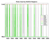
Fig 2: How AUDOU change her mind.

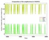
Fig 3: Distributions of metarules in AUDOU's neighborhood.

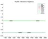
Fig 4: AUDOU's neighbors payoffs.

Fig 5: Evolution of the proportions of imitations rules. (click to enlarge)

Fig. 7: Clutering rates for imitation rules.

fig. 8: mean rate of cooperation per imitation rule.

Fig 9 : mean payoffs per imitation rule.

Fig 10: mean payoffs per action.